on
Shocks
Intro and Shocks Discussion
Since Election Day is 13 days away, I will mainly focus this blog post on refining my current models at the nationwide and district level. However, I will also include a brief summary of this week’s topic, Shocks, as I think it is important in considering uncertainty in my models.
Election shocks can be described as events that one couldn’t have forecasted but could significantly affect election outcomes. In this year specifically, the Dobbs decision to overturn Roe v. Wade, the war in Ukraine, and the Mar-a-Lago investigation are considered shocks to the 2022 election. It is challenging to estimate the precise impacts of a given shock because we do not run elections prior and after, but polls (generic and candidate-based) often capture the ways in which the shock might have affected public opinion.
In my models, I do not plan to incorporate data about the effects of shocks, largely because it is unclear which shocks (if any) may occur between now and the election. Yet, I think this topic is very important to mention because it adds further uncertainty to the prediction estimates and demonstrates how elections do not occur in a vacuum, but rather in a complicated geopolitical setting where fundamental trends may not hold.
Model Update
I have chosen against using a pooled model for my final prediction because I have decided to do a nationwide rather than district-level analysis. In this way, myn model represents an aggregated rather than pooled approach.
I have decided to stick with the nationwide approach because I am not confident enough in my district-based data to generate 436 unique predictions. Parituclarly with the redistricting in 2021, a district’s previous makeup and voteshare can vary significantly for the upcoming cycle. As well, there are a few new districts created, of which my only data would be from expert ratings.
I believe that using an aggregated US seatshare model is more within the scope of my data. I will build models for both predicting nationwide seat share and voteshare. Additionally, I will perform specific district-based analysis for my district, Ohio-01, because i am confident in the level of polling and information about this area.
Nationwide Model Update
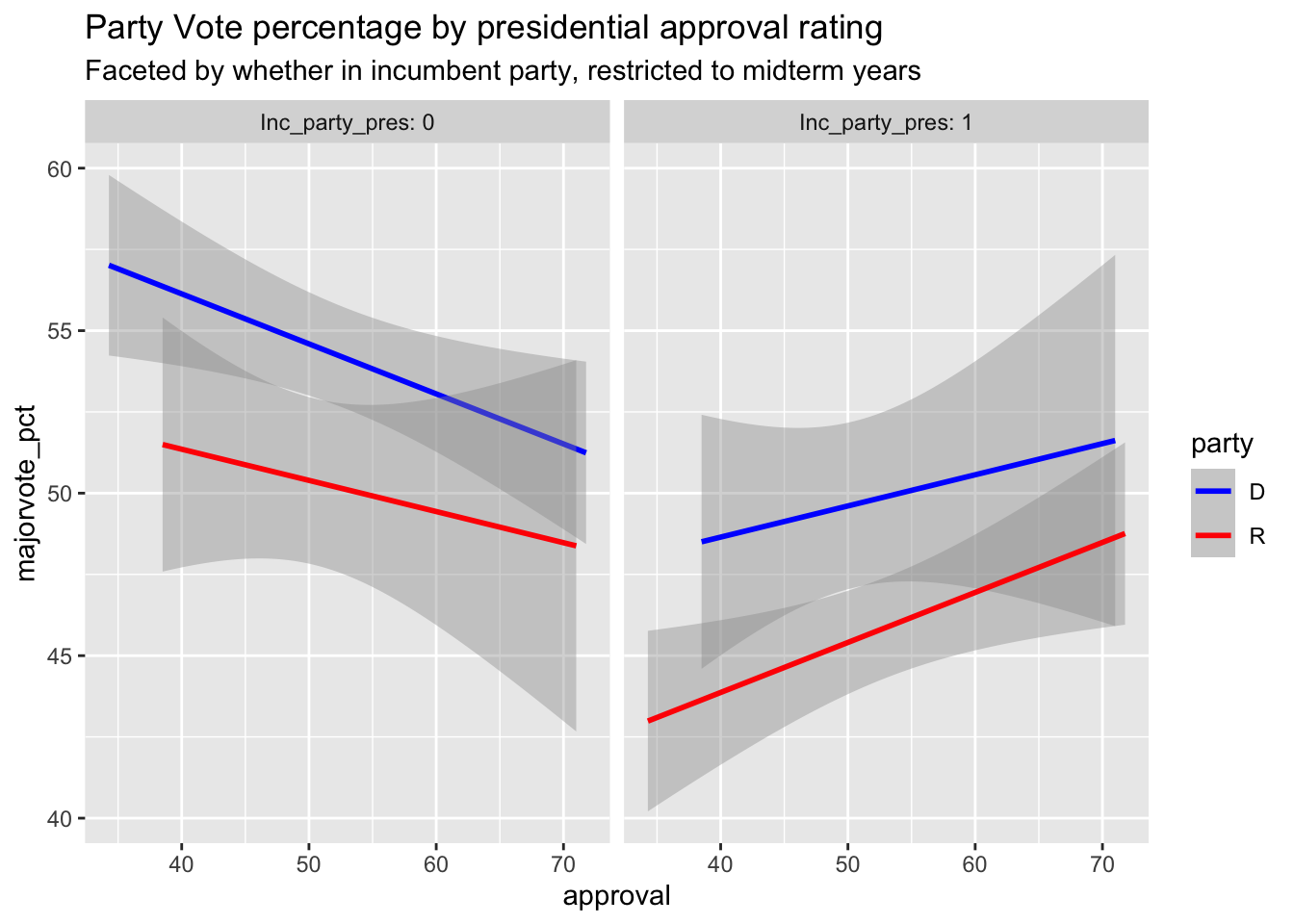 In this plot, we see that for candidates of the same party as the President during midterm years, their vote share is postiively correlated with the president’s approval. On the other hand, candidates
of opposite parties as the President are negatively correlated with approval. This intuitively makes sense,
so I included it in my national model below.
In this plot, we see that for candidates of the same party as the President during midterm years, their vote share is postiively correlated with the president’s approval. On the other hand, candidates
of opposite parties as the President are negatively correlated with approval. This intuitively makes sense,
so I included it in my national model below.
Here, I have built linear models for the popular vote and seat share for each party using fundamental data (incumbency, president party), polling (generic, president), and economic data (gdp growth).
##
## ==========================================================
##                                   Dependent variable:
##                               ----------------------------
##                                   seats      majorvote_pct
##                                    (1)            (2)
## ----------------------------------------------------------
## Inc_party_pres                  -82.476***     -8.512***
##                                  (16.156)       (2.145)
##
## MidtermYear                      14.309**       2.123**
##                                  (5.314)        (0.788)
##
## approval                        -0.757***      -0.084***
##                                  (0.186)        (0.026)
##
## GDP_growth_pct                   -1.220**       -0.111
##                                  (0.514)        (0.071)
##
## poll_pct                         1.928***      0.292***
##                                  (0.475)        (0.065)
##
## lag_seats                        0.648***
##                                  (0.071)
##
## lag_pv                                         0.401***
##                                                 (0.101)
##
## Inc_party_pres:MidtermYear      -27.759***     -4.322***
##                                  (7.830)        (1.221)
##
## Inc_party_pres:approval          1.496***      0.166***
##                                  (0.308)        (0.041)
##
## Inc_party_pres:GDP_growth_pct    2.042***        0.170
##                                  (0.723)        (0.102)
##
## Constant                         32.954*       21.296***
##                                  (17.902)       (3.753)
##
## ----------------------------------------------------------
## Observations                        51            51
## R2                                0.923          0.858
## Adjusted R2                       0.906          0.827
## Residual Std. Error (df = 41)     11.263         1.570
## F Statistic (df = 9; 41)        54.763***      27.584***
## ==========================================================
## Note:                          *p<0.1; **p<0.05; ***p<0.01
As the model output shows, almost all variables are significant at the 5% level. I chose to use multiple interactions to account for the cases where the candidate represents the same, or different, party as the sitting president.
My data is structured in a long format, such that the unit of measurement is by party*year Hence, for every year, there are 2 observations separated by party.
Model Validation
## # A tibble: 2 × 4
## party year pred_seats[,"fit"] [,"lwr"] [,"upr"] pred_vote[,"fit"] [,"lwr"]
## <chr> <dbl> <dbl> <dbl> <dbl> <dbl> <dbl>
## 1 D 2022 198. 174. 223. 47.7 44.4
## 2 R 2022 240. 215. 264. 52.5 49.1
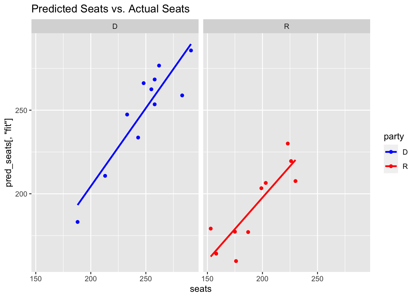
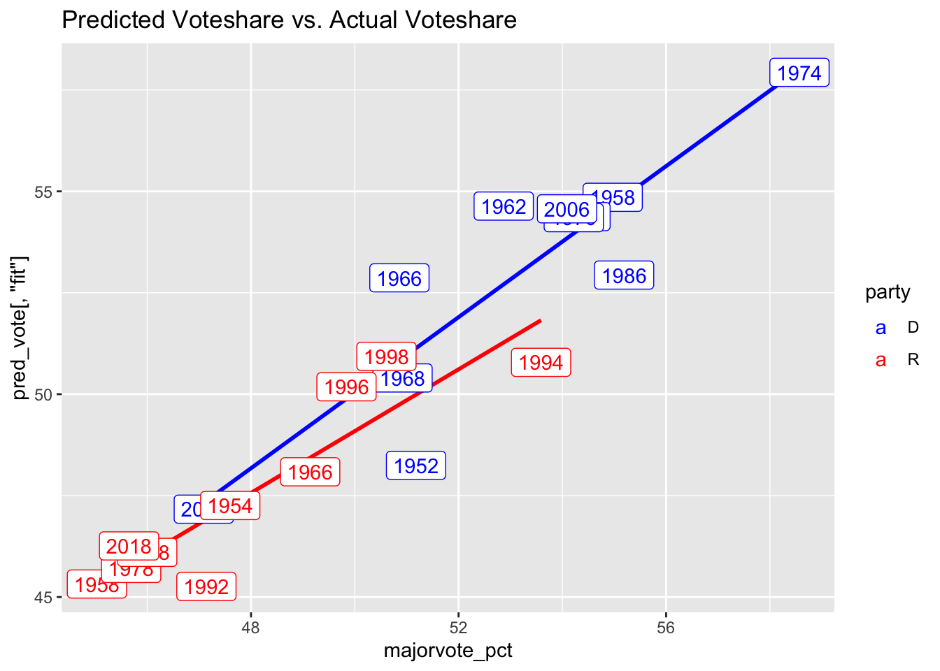
## # … with 1 more variable: pred_vote[3] <dbl>As the graphs above show, the model fits fairly well across the testing dataset. And, the prediction for 2022 is that the Democrats will get 198 seats with the Republicans receiving 240 seats. This sum (438) is greater than the total sum of seats (436), so I will work on considering how to best account for this constraint. Similarly, my model predicts that Republicans will get about 52.5% of the vote while Democrats will receive about 47.7% of the vote. The confidence intervals are fairly large and just barely overlap, suggesting that both predict with strong confidence that the Republicans will gain a majority over the Democrats this November.
Moving forward, I will work on building simulations to better quantify the uncertainty provided by my simulations.
Ohio section
Here, I provide an update to my Ohio district analysis. Similarly, it is structure din the long format with the unit of analysis at the candidate*year. One important data choice was that I removed uncontested races, but included a term for whether the prior election was uncontested.
##
## ==================================================
##                            Dependent variable:
##                        ---------------------------
##                                   pv2p
## --------------------------------------------------
## StatusIncumbent                 10.909***
##                                  (2.392)
##
## prev                            0.284***
##                                  (0.095)
##
## same_party:MidtermYear           -3.709
##                                  (2.463)
##
## Constant                        32.191***
##                                  (4.361)
##
## --------------------------------------------------
## Observations                       70
## R2                                0.472
## Adjusted R2                       0.448
## Residual Std. Error          8.482 (df = 66)
## F Statistic              19.648*** (df = 3; 66)
## ==================================================
## Note:                  *p<0.1; **p<0.05; ***p<0.01
Prediction Interval
oh_22$pred<-predict(lm_oh,oh_22,interval='prediction')
oh_22[,c(1:3,7:9)]
## # A tibble: 2 × 6
## year party term same_party party_support pred[,"fit"] [,"lwr"] [,"upr"]
## <dbl> <chr> <dbl> <dbl> <dbl> <dbl> <dbl> <dbl>
## 1 2022 R 16 0 45.3 58.4 41.1 75.6
## 2 2022 D 0 1 44.7 41.6 24.2 59.1This model for Ohio-01 predicts that Incumbent Steve Chabot (R) will receive about 65% of the vote, while challenger Greg Landsman (D) will get about 42% of the vote. This is very different from the few polls that have been released, suggesting each candidate is at about 47% of the vote. However, the confidence intervals are very large, so similar to my earlier section, one of my next steps will be to better quantify the confidence intervals. Additionally, I will work on building more of a training/testing split to better validate this model and reformatting for my predictions.
This difference between my prediction and the polls may be due to the recent redistricting that my model hasn’t accounted for, polling errors, or entirely other causes. Moving forward, I will work on improving my Ohio model to include a mixture of polling/expert ratings. I was having trouble with this because there are so few years that have data with this information.