on
Ground Game
Intro
In this blog post, I look into the “Ground Game,” or the non-ad components to political US House campaigns. Primarily, I focus on Extension #2 whether expert predictions (blog post 4) and ad spending (blog post 5) affect turnout at the district level. I only end up finding a visual correlation between turnout and ad spending. I end with an update to my model where I work on district and nation-level outcomes.
There is mixed academic literature on whether the campaign’s ground efforts have a tangible impact on the success of the candidate. In Enos and Fowler’s article, they find that presidential campaigns can increase the turnout by 7-8 percentage points, exploiting media market spillovers. In this blog post, I do not have a comparable research design, but rather look through some aggregate data to explore the topics descriptively.
Ads
To begin, I examine whether there is a relationship between expert predictions and turnout. I run three models, as shown below, with each model adding a variable.
In my first model, I simply run turnout, calculated as total voters minus the district’s eligible citizens of that age group, on the average expert prediction rating. One immediate limitation in this data is that there were only 390 observations for which I had expert predictions between 2010-2022, so the training dataset becomes 270 observations. The next model also includes a variable for the status of the incumbent, and the final model includes a variable for the presidential party.
##
## ==================================================================================
##                                          Dependent variable:
##                     --------------------------------------------------------------
##                                                turnout
##                             (1)                  (2)                  (3)
## ----------------------------------------------------------------------------------
## avg_rating                -0.006              -0.013**              -0.013**
##                           (0.004)              (0.005)              (0.005)
##
## RepStatusIncumbent                             0.041**              0.042**
##                                                (0.019)              (0.019)
##
## president_partyR                                                     -0.002
##                                                                     (0.016)
##
## Constant                 0.585***             0.594***              0.594***
##                           (0.019)              (0.020)              (0.020)
##
## ----------------------------------------------------------------------------------
## Observations                270                  270                  270
## R2                         0.008                0.026                0.026
## Adjusted R2                0.005                0.019                0.015
## Residual Std. Error  0.123 (df = 268)     0.122 (df = 267)      0.122 (df = 266)
## F Statistic         2.248 (df = 1; 268) 3.602** (df = 2; 267) 2.396* (df = 3; 266)
## ==================================================================================
## Note:                                                  *p<0.1; **p<0.05; ***p<0.01
## lm1 lm2 lm3
## rmse 0.01230225 0.01161154 0.01157815
## mae 0.08840246 0.08660321 0.08656715As the model output shows, my first model does not find there to be a significant relationship between the turnout and average rating. However, after controlling for incumbency, both models 2 and 3 determine that there is a negative relationship between the two variables. This means that as Cook predicts that a district will turn more Republican, the turnout is predicted to be about .01 points lower. Hence, the relationship is still about neglegible.
Next, I created a small table with rmse and mae outputs as validation tests on my testing data. Each of these measures is pretty similar, suggesting that even though our adjusted R^2 was much better after including incumbency data, the test data didn’t show large differences.
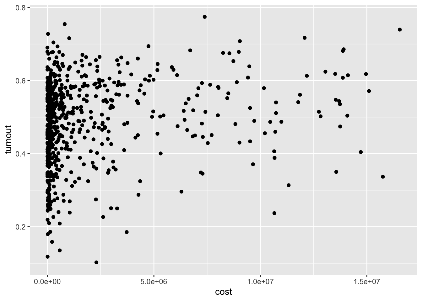
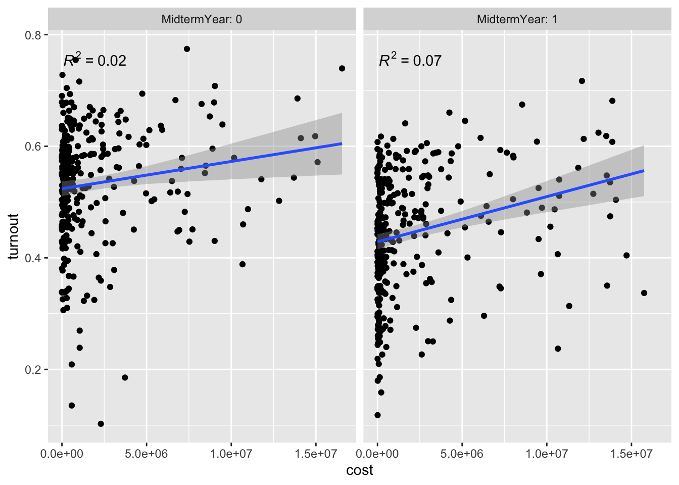
To continue looking at turnout data, I examine the relationship between total $’s spent on ads (for districts with data) and turnout in districts between 2010 and 2022. This leads to 770 total observations. As this first graph shows, there appears to be a positive, but noise, correlation between ad spending and turnout, giving beginning evidence that ad spending is effective at mobilization. To control for midterm years, I next facet it by whether or not the election was during a midterm year. I find that the R^2 is slightly better after faceting, but the correlation is likely still hard to tease out without further data.
#ii.
#Overall model
Instead of going deeper into models for any of these relationships, I will return to my existing model. Since these variables (turnout and ads) are hard to predict ahead of time, I am going to stick to fundamental-based data in my model for now.
One of the main challenges has been cleaning and merging the district-level data to get a clean dataset of past results and the 2022 races. This week, I have been working to bind historical data to 2022 data but am encountering a few issues, including: names being formatted in different ways, how to treat races where there are more than one party from a specific race (eg. Alaska House), and districts that have recently been drawn (eg. Colorado District 8).
Hence, I am going to return to my nationwide model where I am more confident that these errors will be diluted. Here, I begin to look at seat share versus fundamental data (house majority incumbency party), economic data (disposable change in income), as well as generic ballot approval ratings. I subset to only midterm years where each row represents the party by year with information, which only amounts to about 30 observations (goes back to 1960).
##
## =======================================================================
##                                        Dependent variable:
##                           ---------------------------------------------
##                                               seats
##                                    (1)                    (2)
## -----------------------------------------------------------------------
## partyR                          -78.909***             -57.142***
##                                  (7.840)                (9.366)
##
## H_incumbent_partyR              -53.818***             -46.103***
##                                  (9.917)                (8.904)
##
## DSPIC_change_pct                                         1.094
##                                                         (1.886)
##
## poll_pct                                                2.226***
##                                                         (0.660)
##
## partyR:H_incumbent_partyR       106.709***             89.149***
##                                  (14.024)               (13.210)
##
## Constant                        256.818***             148.610***
##                                  (5.544)                (32.450)
##
## -----------------------------------------------------------------------
## Observations                        32                     32
## R2                                0.793                  0.856
## Adjusted R2                       0.770                  0.828
## Residual Std. Error          18.386 (df = 28)       15.915 (df = 26)
## F Statistic               35.676*** (df = 3; 28) 30.841*** (df = 5; 26)
## =======================================================================
## Note:                                       *p<0.1; **p<0.05; ***p<0.01
Through these initial results, it appears as though adding data about the generic polling percentage and disposable income create better predictions to my model. Moving forward, I would like to add lagged presidential data so I can better use presidential approval data.
Conclusion:
This week was very focused on coding, cleaning, and preparing datasets for further models. Hence, my output is not as long or detailed as in most weeks. However, the blog extension gave interesting insights into the potential relationships that exist between the perceived closeness of a race(expert prediction), campaign ad spending, and turnout figures.
Moving forward, I will be focused on improving my nationwide model, particularly in considering whether to include all years (not just midterms), and how to best incorporate different forms of data. Additionally, I will work on cleaning my district-wide dataset so it is more fit for models.
Citations
Ryan D. Enos and Anthony Fowler. Aggregate Effects of Large-Scale Campaigns on Voter Turnout. Political Science Research and Methods, 6(4):733–751, 2016.